SARS-CoV-2 evolution on a dynamic immune landscape

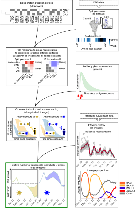
DMS data

We used all DMS data^5,17 available on 13 February 2023 to assess the phenotype (escape from neutralizing antibodies) of each SARS-CoV-2 variant. DMS measures, in a yeast-display assay, how much a mutated site s in the RBD affects the binding of antibodies elicited by a variant that is not mutated at site s. We utilized data from 836 antibodies that were classified into 12 distinct epitope classes^17,18 (see below) and aggregated all values on site level by their mean, yielding ‘escape fractions’ to antibody a for each mutated site ef_s,a (values were bounded at 0.99). Escape fractions denote a proxy for quantifying the probability that an antibody does not bind an RBD that contains an alteration at site s. Thus, the numerical value depends on the antibody potency, and hence we aimed to convert these values to ‘fold resistances’ (fold change in antibody potency; see also Extended Data Fig. 1a–c). Assuming that mutational effects of site s on the binding affinity are independent, the binding probability of an antibody elicited by a variant x to a variant y can be expressed as

in which ef_s,a is the normalized escape fraction of mutated site s with respect to antibody a, and \(\varOmega (x,y)\) denotes the set of RBD sites that distinguish variants x and y (ref. ¹⁷). Using classical pharmacodynamic approaches, we then model the binding probability as

in which FR_x,y(a) denotes the fold resistance of variant y to an antibody a elicited by variant x. The parameter \({{\rm{IC}}}_{50({\rm{DMS}})}(a)\) corresponds to the half-maximal inhibitory concentration (that is, ‘potency’) of the antibody against the antibody-eliciting variant, which was extracted from the DMS dataset. Notably, c_a = 400 μg ml⁻¹ was the antibody concentration at which the DMS experiment was conducted^4,18. Combining equations (1) and (2) yields:

As already evident from Extended Data Fig. 1a–c, DMS estimates of ef_s,a, as well as the corresponding FR_x,y(a), can become unreliable depending on antibody concentrations and antibody potency \({{\rm{IC}}}_{50(x)}(a)\), falsely predicting hyper-susceptibility (FR_x,y(a) < 1). We enforce that FR_x,y(a) ≥1 to avoid such artefacts.

Epitope classes

On the basis of the similarity of antibody profiles in DMS data, antibodies were previously classified into 12 epitope classes (A, B, C, D1, D2, E1, E2.1, E2.2, E3, F1, F2, F3)¹⁸ (Supplementary Tables 1 and 2). As we encountered more than 30% missing values for epitope classes E2.1 and E2.2, we merged them with E1 into a new class (E12), as they bind to similar regions, including amino acid site R346 (ref. ⁴²). Finally, we retrieved a matrix of 10 epitope classes Α = (A, B, C, D1, D2, E12, E3, F1, F2, F3) for 179 RBD sites. This classification indicates that antibodies belonging to the same class bind to overlapping epitopes, and there is little overlap between epitope classes (Fig. 2a). Consequently, we assumed that antibodies within the same epitope class would be similarly affected by RBD alterations, whereas phenotypic changes between epitope classes may vary considerably.

We then quantified the fold resistance associated with each epitope class as the average fold resistance of all antibodies belonging to the class

for all epitope classes \({\vartheta }\) in Α (Fig. 2a).

As a proof of concept, we compared DMS-derived FR_x,y(\({\vartheta }\)) using the calculations above with fold resistance values obtained from virus neutralization assays (reported in ref. ⁴²) for antibodies targeting all epitope classes Α defined above. As can be seen in Extended Data Fig. 1d, we observed a strong and significant positive correlation between the DMS-derived FR_x,y(\({\vartheta }\)) and those obtained by neutralization assays and reasonable agreement for polyclonal sera (Extended Data Fig. 1e–g).

As the DMS experiments were generated only for RBD-targeting antibodies, no escape data were available to quantify the fold resistance of NTD-targeting antibodies. To overcome this limitation, we included an additional class of NTD-targeting antibodies targeting three antigenic super-sites⁴³: spike amino acid positions 14–20, 140–158 and 245–264. Consequently, we assigned alterations in the antigenic super-sites fold resistance values of 10, which is in range with corresponding ELISA experiments⁴³. However, the model can be updated if comprehensive DMS data for the NTD domain become available⁴⁴.

Assuming independence between mutational effects, the total fold resistance of a variant y to binding of an NTD-targeting antibody elicited by a variant x was computed as:

in which |Ω(x, y)| denotes the number of mutational differences between variants x and y in the antigenic super-site of the NTD.

Variant cross-neutralization probability

We assumed that a virus is neutralized if at least one antibody is bound to its surface (either at the RBD or NTD of the spike protein). Here, we collectively consider all antibodies from the same epitope class as they compete for the same binding site. By assuming binding independence between epitope classes, the neutralization probability can be computed as:

with \({b}_{{\vartheta }}(t,x,y)\) denoting the probability that an antibody of epitope class \({\vartheta }\) in Α ∪ (NTD) binds to the virus with

in which \({c}_{{\vartheta }}(t)\) is the antibody’s concentration in an individual at time t, \({{\rm{IC}}}_{50(x)}({\vartheta })\) is the half-maximal inhibitory antibody concentration against the variant that elicited the antibody. FR_x,y(\({\vartheta }\)) is the fold resistance of variant y to binding of antibodies of epitope class \({\vartheta }\), elicited by variant x.

Antibody potency

Next, we quantified \({{\rm{IC}}}_{50(x)}({\vartheta })\) for each epitope class. As the DMS data were derived from yeast-display RBD mutant libraries, absolute antibody potencies may not directly translate to a clinical setting. However, the ranking of antibody potencies may be preserved. Consequently, we estimated the relative potency D(\({\vartheta }\)) from the DMS data:

in which \({\vartheta }\in {\rm{A}}\), and \(\widehat{\,{{\rm{IC}}}_{{50}_{({\rm{DMS}})}}}({\vartheta })\) denotes the average potency of all antibodies belonging to epitope class \({\vartheta }\). Epitope-class-specific clinical antibody potency \({{\rm{IC}}}_{50(x)}({\vartheta })\) was then inferred using the following relation:

in which \(\widehat{\,{{\rm{IC}}}_{{50}_{(x)}}}\) denotes the \({{\rm{IC}}}_{50(x)}\) averaged over all epitope classes. NTD-targeting antibodies were not included in the DMS dataset, and hence we set

\(\widehat{\,{{\rm{IC}}}_{{50}_{(x)}}}\) was the only free parameter in the model, which we estimated by fitting our model to (Wuhan-Hu-1-strain) vaccine efficacy (VE) data against the Delta lineage (B.1.617.2) present between 4 July 2021 and 31 December 2021 (Fig. 2d; genomic profile in Supplementary Table 3).

We considered interindividual differences in antibody pharmacokinetics (see below), implemented as combinations of the parameters t_max (time of maximal antibody concentration) and t_half (antibody half-life). For parameter estimation, we first estimated optimal drug potencies \(\widehat{\,{{\rm{IC}}}_{{50}_{(x)}}}\) (t_max, t_half) for each t_max, t_half combination in a 5 × 15 grid (ranges below) and then averaged over these 75 estimates. Parameter estimation was performed using scipy.optimize.root, applying the Levenberg–Marquardt method to solve the ordinary least-square problem.

in which VE(t, Wuhan-Hu-1, Delta) denotes the vaccine efficacy against the Delta strain t days after antigen exposure with the Wuhan-Hu-1 strain. Here, we assumed that VE = infection risk reduction ≈ P_Neut.

As a proof of concept, we then tested our predictions with Wuhan-Hu-1-strain VE data against Omicron infection (Fig. 2d; genomic profile in Supplementary Table 3). Utilized VE data include those from all studies in which Wuhan-Hu-1-strain vaccines were tested and which were computed on the basis of hazard ratios or rate of confirmed infection (Supplementary Tables 4 and 5).

Antibody pharmacokinetics

To determine the duration of sterilizing immunity against any variant y, we accounted for antibody pharmacokinetics (PK) after antigen exposure to variant x (by means of infection or vaccination). Pharmacokinetics were considered using a classical, descriptive linear model with an analytical solution

in which t denotes the time after antigen exposure and c(t) denotes the normalized (fraction of maximum) concentrations of the antibody. The parameters k_e and k_a (elimination and ‘absorption’ parameters in classical PK models) were related to known quantities through established PK relations; that is,

In our simulations, we considered identical PK for antibodies of the different epitope classes. Utilized parameters (t_max, t_half) were extracted from the literature: the time of maximal antibody concentrations (t_max) varied between 14 and 28 days after antigen exposure^26,45,46, and the half-life (t_half) ranged between 25 and 69 days^{19,47,48,49,50,51,52,53}. For simulation, we used different combinations of (t_max, t_half) in a 5 × 15 grid within a range of t_max within 14 to 28 days and t_half within 25 to 69 days and plotted the range of predictions (minimum, maximum).

SARS-CoV-2 genomic data

We collected SARS-CoV-2 genomic data from Germany published by the Robert Koch Institute, including only genomic data from the ‘random sampling’ strategy, which denotes most of the sequence data. For other countries (Australia, Brazil, Canada, Denmark, France, Japan, Mexico, South Africa, Sweden, the UK and the USA), we downloaded data from GISAID (https://gisaid.org); however, here we could not be sure that the data are representative (randomly sampled), as anyone can upload SARS-CoV-2 data to GISAID. A dataset summary is given in Supplementary Table 6.

Variant proportions and spike pseudo-groups

If pangolin lineage information was absent in the data, lineage information was assigned using established methods^54,55. Alteration profiles for all sequences were extracted using covSonar. For each lineage, we collected all ‘characteristic’ spike amino acid changes in the RBD (amino acid position 331–541) and the NTD antigenic super-sites regions (amino acid positions 14–20, 141–158 and 245–264) for subsequent analyses. In our work, ‘characteristic’ implied that an amino acid change was present in at least 75% of all sequences from that lineage. The ‘antigenic profile’ for each lineage was then determined on the basis of the set of unique alterations within the NTD and RBD regions. Differences between lineages were defined as the set difference between alteration profiles. Clustering lineages with identical ‘antigenic profiles’ yielded spike pseudo-groups with distinct genomic profiles in the RBD and NTD region of the spike protein. On the basis of the genomic profiles and their clustering into spike pseudo-groups, we computed pseudo-group frequencies π_x(t) for all x ∈ \({\mathcal{X}}\) in the entire observation horizon. The frequencies were computed such that there were at least 100 sequences per time step, and daily lineage frequencies were computed by using linear interpolation between time steps. Furthermore, we filtered out spike pseudo-groups that never reached levels of >1% frequency to reduce noise from sequencing errors. Data files with lineage and pseudo-group frequencies and alteration profiles for all countries are available via GitHub at https://github.com/KleistLab/VASIL (a summary is given in Supplementary Table 6).

Genome-based reconstruction of infection timeline

Unfortunately, the infection timeline cannot be reconstructed from reported cases, as test coverage and reporting of SARS-CoV-2 became increasingly unreliable. To overcome this data limitation, we recently developed the genome-based incidence estimator, GInPipe²². This computational pipeline reconstructs the infection timeline solely from time-stamped viral sequences. Owing to the short infectious phase of SARS-CoV-2 (ref. ⁵⁶), a limited amount of intra-patient evolution is typically observed before an infection is passed on. This implies the existence of an ‘evolutionary signal’ ϕ that relates haplotype diversity and the number of alterations present in a temporal collection of viral sequences to the number of infections (see ref. ²² for details). We confirmed previously that this evolutionary signal is proportional to the actual number of infected individuals I(t) ≈ cϕ(t) at time t.

Although GInPipe works quite robustly when sequencing efforts change over time, extreme changes may cause biases²². For the USA and the UK, we observed major drops in the number of available sequences (≈10-fold after 2022), and henceforth downsampled the number of viral sequences to 6,000 and 2,500 per day, respectively, which corresponds to the maximum number of sequences after the drop in sequencing efforts (Extended Data Fig. 5).

In the pipeline, sequences are pooled according to their collection date, such that ‘bins’ b comprise either the same number of sequences n_b or span the same number of days ∆d_b. We chose time spans ∆d_b = 7, 10 and 14 days and bin sizes of n_b = 2% and 5% of all sequences, as well as the average weekly number of sequences for each particular country. Incidence correlates ϕ_b were filtered out if the time span of a bin was smaller than 3 days, or if a bin comprised fewer than 50 sequences. We allowed a bin to span at most 21 days (data-rich setting) or as many days as necessary to comprise the minimal number of sequences (data-poor settings). Bin-wise ϕ_b estimates were smoothed using kernel smoothing with a bandwidth of 14. GInPipe-estimated incidence correlates are depicted in Extended Data Fig. 5 for all investigated countries.

To confirm the validity of GInPipe-estimated incidences, we compared our predictions with other unbiased incidence measures for Germany (citizen science and wastewater data; Extended Data Fig. 3) and with a UK dataset from the representative COVID-19 Infection Survey of the Office for National Statistics (ONS)⁶, using the percentage of infected individuals in the UK from the ONS study as the ground truth (March 2021–March 2023; Extended Data Fig. 4).

The percentage of PCR-positive individuals from GInPipe at the time point of interest was then computed using a rolling sum over 10 days⁵⁶, and normalized with the ratio of the population size and the sum of infected people in the respective time horizon according to the ONS. For the reported cases, the rolling sum over 10 days was normalized by the population size of the UK.

Expected sterilizing immunity against variant y

The estimation of cross-neutralization probability P_Neut enabled us to estimate the expected number of individuals being immune against infection with a variant y for a given time point t by taking the infection history before time t into account. The expected number of individuals immune to infection with strain y is given by

in which \({\mathcal{X}}\) denotes the set of all variants present within the time horizon of interest, P_Neut(t − s, x, y) denotes the probability that an infection with strain x, that occurred t − s days ago cross-neutralizes a variant y. In the equation above, π_x(s) denotes the proportion of variant x at day s < t, derived from the molecular surveillance, and I(t) denotes the number of infected individuals at some previous time point s. The expected number of susceptible individuals to a variant y at time t can then be calculated as \({\mathbb{E}}[{{\rm{S}}}_{y}(t)]={\rm{Pop}}-{\mathbb{E}}[{{\rm{Immune}}}_{y}(t)]\), in which Pop denotes the total population size. The variable I(s) is typically not available, but can be replaced by incidence correlates ϕ(s) = I(s)/c (see below).

Variant dynamics

To estimate whether an emerging variant may successfully out-compete existing variants, we estimated the relative growth advantage of a variant γ_y(t):

in which the denominator denotes the average growth rate across all variants existing at time t and for which α_x > 0 denotes a variant’s intrinsic (antibody-independent) relative transmission fitness, which we assumed to be nearly identical for all circulating variants α_x ≈ α, implying that variant dynamics are dominated by infection history and immune dynamics. We ignored low-abundance variants with π_x(t) < 1% and renormalized accordingly. We computed the frequency-weighted average γ_z(t), whenever different variants were combined during analyses (as indicated in the respective graphics).

Replacing infection numbers with incidence correlates

As infection numbers I(t) are typically unreliable, our method can utilize any incidence correlate, such as GInPipe’s ϕ(t), wastewater virus load trajectories or reliable estimates from large citizen science projects. With regard to GInPipe’s output, we showed in Extended Data Figs. 3 and 4 and in ref. ²² that I(t) ≈ cϕ(t), which allows us to use ϕ(s) instead of the number of infected individuals I(s) when computing \({\mathbb{E}}[{{\rm{Immune}}}_{x}(t)]\), as performed in Figs. 3–5. To compute \({\mathbb{E}}[{{\rm{S}}}_{x}(t)]\), we can write \({\rm{Pop}}=k\cdot \int I(s){\rm{d}}s\approx k\cdot c\cdot \int \phi (s){\rm{d}}s\), for which k > 0 is a scaling factor (for example, k⁻¹ = 2 implies that every individual got infected twice, on average, over the time horizon of interest). When reconstructing actual incidences for Germany and the UK, we found that k ≈ 1 for the length of the time horizon (Extended Data Fig. 9). k is a modelling choice and any mis-estimation of k affects only the scaling of γ_y(t) (Extended Data Fig. 10). Qualitative results (inflection points γ_y = 0; variant ‘growth’ γ_y > 0; variant ‘decline’ γ_y < 0) remain unaffected. The interpretation of this ‘scaling’ is straightforward: if one overestimates the number of individuals that became infected, one under-predicts the number of susceptible individuals and thus infers stronger competition among variants, which is expressed in overestimation of the amplitude of γ_y(t) by some constant ξ > 1.

Relation of γ
_y to variant dynamics

In a discrete-time quasi-species model⁵⁷, the theoretical variant frequencies \({\boldsymbol{p}}\in {[\mathrm{0,}1]}^{|{\mathcal{X}}|}\) are given by

for which \({\boldsymbol{Q}}\in {{\mathbb{R}}}^{|{\mathcal{X}}|\times |{\mathcal{X}}|}\) denotes a transition matrix between different variants, which we set to the identity matrix Q = Id, ignoring any mutational transitions from one variant to another. Fitness values of any variant y, relative to the population average \(\bar{f}(t)=\,{\sum }_{x}{p}_{x}(t)\cdot {f}_{x}(t)\) are contained in matrix \({\boldsymbol{F}}(t)={\rm{diag}}([\ldots ,\,{f}_{y}(t)/\bar{f}(t),\,\ldots ])\). Consequently, for p_y(t) > 0, we get

if fitness is determined by population immunity.

Modelling booster vaccinations in Germany

As the vaccination timeline contains the number of individuals that were vaccinated, we first reconstructed actual infection numbers for Germany using GInPipe²²: we inferred the time-dependent case ascertainment probabilities P_rep(t) ≤ 1 (that is, the probability of an infection being reported):

for which I_rep(t) ≤ I(t) denotes the daily reported infections (weekly cases/7). We smoothed reported cases I_rep(t) with a bandwidth of 14.

Last, we normalized the case ascertainment probabilities \({\widetilde{P}}_{{\rm{rep}}}(t)\) at maximum to be able to estimate the minimum number of infections I_min(t)

The minimum number of infections is then calculated as

The impact of infections on the immune landscape was then modelled as outlined above by setting I(t) ≈ I_min(t). To model the impact of booster vaccinations in Germany (Extended Data Fig. 7), we added exposure to either the Wuhan-Hu-1-variant antigen or the BA.4 + BA.5-variant antigen corresponding to the timeline of vaccination (https://impfdashboard.de/en/) to the infection timeline and computed the relative fitness γ_y(t) on this basis. Note that this reconstruction of actual infection numbers can become unstable, as it is normalized to an extreme point (the maximum) and therefore warrants post-analysis inspection. Moreover, it requires the use of case reporting data, which largely ceased by the end of 2023.

Reporting summary

Further information on research design is available in the Nature Portfolio Reporting Summary linked to this article.